Testing The Limits on Wealth Inequality
In this post, I pointed out that we are going to see an empirical test of Piketty’s theory of rising wealth inequality. The theory itself is not well understood, and Piketty has revisited it since the publication of Capital in the Twenty-First Century, and published an economist’s dream of a paper in full mathematical glory here. The American Economics Association devoted space in its journal to arguments about the theory, giving Piketty an opportunity to discuss his theory in what I think is a very readable paper, and one worth the time.
He starts by saying that the relation between r, the rate of return to capital, and g, the rate of growth in the overall economy, are not predictive. They cannot be used to forecast the future, and are not even the most important factor in rising wealth inequality. The crucial factors are institutional changes and political shocks. Neither can the relation tell us anything about the decrease in the labor share of national income. He points to supply and demand for skills and education in this paper, as he does in his book, but this is a at best an incomplete explanation, owing more to the neoliberal view that the problems of workers are their fault than to a clear understanding of social processes in the US. A better explanation lies in tax law changes, changes in labor law and enforcement of labor law, rancid decisions from the Supreme Court, failure to update minimum wage and related laws, and government support for outsourcing and globalization.
What the theory does say is the subject of Part II.
I now clarify the role played by r > g in my analysis of the long-run level of wealth inequality. Specifically, a higher r − g gap will tend to greatly amplify the steady-state inequality of a wealth distribution that arises out of a given mixture of shocks (including labor income shocks).
In other words, as the raw number r – g increases, wealth inequality reaches a limit at a higher level, and income and wealth mobility become lower.
The important point is that in this class of models, relatively small changes in r − g can generate large changes in steady-state wealth inequality. For example, simple simulations of the model with binomial taste shocks show that going from r − g = 2% to r − g = 3% is sufficient to move the inverted Pareto coefficient from b = 2.28 to b = 3.25. Taken literally, this corresponds to a shift from an economy with moderate wealth inequality — say, with a top 1 percent wealth share around 20–30 percent, such as present-day Europe or the United States — to an economy with very high wealth inequality with a top 1 percent wealth share around 50–60 percent, such as pre-World War I Europe.
The inverted Pareto coefficient β is a measure of inequality used by Piketty and his colleagues. Here’s how he explains it in this paper:
That is, if β = 2, the average income of individuals with income above $100,000 is $200,000 and the average income of individuals with income above $1 million is $2 million. Intuitively, a higher β means a fatter upper tail of the distribution. From now on, we refer to β as the inverted Pareto coefficient.
The theoretical basis for this result can be found here, where Piketty and his colleague Gabriel Zucman provide a typical economists mathematical explanation. I’ve read some of this paper, but it is tough going.
The returns to capital, especially business capital, are quite a lot higher than the levels given in Piketty’s example. Here’s the chart:
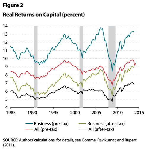
The returns to all capital after tax are about 7%. Paul Krugman put up a blog post saying that a realistic growth rate is about 2.2% at best for the next few years. This gives a difference r – g = 4.8%. Then using the equations on page 1356, we get an estimate that the inverted Pareto coefficient would be in the range of 11, which is a lot higher than the levels Piketty uses in the quoted material. By way of comparison, with that number, the average wealth of people with more than $10 million net worth would be $110 million. In the example Piketty gives for the top .1% with β =3.25, the figure would be $32.5 million.
Piketty notes that these coefficients are a rapidly rising function of r – g, which is apparently the case. In a recent paper, Emmanuel Saez and Gabriel Zucman estimate that the top .1% has a wealth share of 22% as of 2012, and there is every reason to think that has risen.
With Piketty’s general rule standing alone, there is no obvious limit to the level of wealth inequality, but in practice there are many practical reasons that it will level off. Some people will have more children, so the fortunes are divided into smaller shares. Some are lucky in investments and others aren’t. There are external shocks, wars and depressions. There are divorces, which split fortunes. Some people are able to earn high levels of labor income on top of capital income, increasing their wealth. Some die early, so their offspring are forced to spend more of their capital income to preserve their existing level of consumption. Others have expensive tastes and spend too much. These external forces eventually bring about a more or less static level of wealth inequality. Overall, this static level is higher when the fraction g/r is lower.
The time periods in the theoretical models used by Piketty and his colleagues are generational, they run 30 years. The big changes in wealth inequality began in the 70s, I’d guess, but became prominent enough that they were noticed in the late 80s and early 90s as the Reagan/Bush era tax cuts took hold, and regulatory structures were dismantled. By 2000, the final touches of formal deregulation were complete, and the Bush administration stopped enforcing most remaining laws leaving capital accumulation without restraint from legal pressure. It’s been about 15 years with little change, about half a cycle. The results follow the line Piketty and his colleagues predicted, and every year the new data supports their theories.
From this we can see that the coming empirical test is the maximum level of wealth inequality, or to put it another way, it’s a test of the downward pressures on the limits of wealth accumulation.
As a nation we have only taken the smallest possible steps to stem that tide, such as slow increases in the minimum wage, and tiny increases in taxes on the wealthiest to the extent they choose not to evade taxation in all sorts of allegedly legal ways. Neither of the presumptive candidates has any intention of making the kinds of changes necessary to change the outcome.
That brings us to the second empirical test: the level of wealth inequality that a civilized nation will accept before demanding change.
Or maybe the test is whether we are so cowed we won’t ever make any demands on our new lords and masters.
Update: for more on the uselessness of tweaks to the current system, see this interview by the excellent Lynn Parramore with Lance Taylor.